
As we all know, Gradient Descent method is an essential part in machine learning that is used to optimize the distance between predictions and true values. Newton’s Method is one of the most well-known root-finding algorithms in numerical analysis. Though both methods involve computing the first order derivative, they are independent ideas and cannot be confused. What are the differences between Gradient Descent and Newton’s Method? When to use which of them?
Difference 1: Rate of Convergence
Suppose we are given a function $f$ is convex, twice differntiable in $\mathbb{R}^n$, and we want to find the local minimum
\[\begin{equation*} \min_{x\in \mathbb{R}^n} f(x). \end{equation*}\]The Gradient Method:
\[\begin{equation*} x_{k+1} = x_k - h_k f'(x_k),\quad h_k > 0 \end{equation*}\]Newton’s Method:
\[\begin{equation*} x_{k+1} = x_k - [f''(x_k)]^{-1}f'(x_k) \end{equation*}\]Where $k = 0, 1, 2, 3,…$
We can immediately observe that the rate convergence of gradient method is linear, while the Newton’s method is quadratic.
Difference 2: Directions
The direction of updating step of Gradient Method follows along the direction of the gradient, while Newton’s Method follows along the inverse of second order derivative (or Hessian for a linear system). We’ll see from the derivations below.
Let us approximate $f(x)$ with the following:
\[\begin{equation*} \phi_G(x) = f(\bar x) + \left< \nabla f(\bar{x}), x-\bar{x}\right> + \frac{1}{2h}\left\Vert x-\bar x \right\Vert^2, \end{equation*}\]where $h >0$.
\[\implies \phi_G'(x_G^*) = \nabla f(\bar x) + \frac{1}{h}(x_G^*-\bar x) = 0\]Then, the minimum of the function is
\[\begin{equation*} x^*_G = \bar x - h \nabla f(\bar x) \end{equation*}\]Thus, this is the iterate of Gradient Method.
Newton’s Method is derived from Taylor Series Approximation of a twice differentiable function $f$. Let us approximate $f(x)$:
\[\begin{align*} \phi_N(x) &= f(\bar{x}) + \left< \nabla f(\bar{x}), x-\bar{x}\right> + \frac{1}{2}\left< \nabla^2 f(\bar{x})(x-\bar{x}), x-\bar{x}\right>\\ \implies \phi_N'(x_N^*) &= \nabla f(\bar x) + \nabla f(\bar x)(x_N^*-\bar x) = 0 \end{align*}\]The minimum of the function is
\[\begin{equation*} x_N^* = \bar x - \left[ \nabla^2f(\bar x)\right]^{-1} \nabla f(\bar x) \end{equation*}\]Therefore, we got the iterate of Newton’s Method.
Recall the inner product between $x$ and $y$,
\[\begin{align*} \left< x, y \right> &= \sum_{i=1}^n x^{(i)}y^{(i)}, \quad \textrm{where} \quad x, y \in \mathbb{R}^n\\ \left\Vert x \right\Vert &= \sqrt{\left< x, x \right>} \end{align*}\]The gradient by definiton is
\[\begin{equation*} f(x+h) = f(x) + \left< \nabla f(x), h \right> + o(\Vert h\Vert) \end{equation*}\]The coordinate representation of the gradient is
\[\begin{equation*} \nabla f(x) = \left(\frac{\partial f(x)}{\partial x^{(1)}}, \frac{\partial f(x)}{\partial x^{(2)}}, ..., \frac{\partial f(x)}{\partial x^{(n)}}\right)^T. \end{equation*}\]The root gradient comes from the Latin word gradi, meaning “to walk”. In this sense, the gradient of a surface is the rate at which it “walks uphill” [[3]] [3].
The figure below is an example of the convergence of the Gradient Method (black curve) and Newton’s Method (blue curve. However, Newton’s Method converges much faster than Gradient Method by taking a different direction.
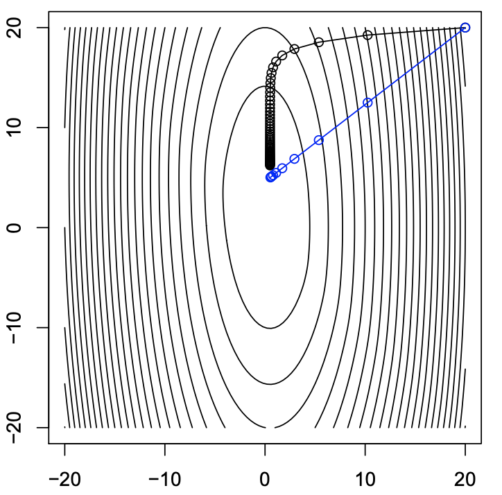
The figure above uses the function $f(x)= (10x_1^2 + x_2^2)/2 + 5\log(1 + e^{-x_1-x_2})$ [[2]] [2].
Difference 3: Operation Time
At each step of iteration of Newton’s Method, we want to compute the Hessian of a $n \times n$ matrix of $f$, this will cost $O(n^2)$ time to compute. The operation time of Gradient Method, however, is $O(n)$ time. If n is a very large number, e.g. n = 1 million, then Newton’s Method is computationally expensive.
Moreover, Newton’s Method converges by one step for a quadratic function.
Consider a quadratic function
\[\begin{equation*} f(x) = \alpha + \left<a, x\right> + \frac{1}{2}\left<Ax, x\right> \end{equation*}\]where $A$ is a symmetric positive definite $n \times n$ matrix.
So
\[\begin{align*} \nabla f(x) &= a + Ax\\ \nabla^2 f(x) &= A \end{align*}\]Then, the minimum of the function is
\[\begin{equation*} x^* =-A^{-1}a \end{equation*}\]We can then see that the direction of Newton’s Method at some $x \in \mathbb{R}^n$ is
\[\begin{equation*} d_N(x)= \left[ \nabla^2 f(x)\right]^{-1} \nabla f(x)= A^{-1}(a+ Ax) = x + A^{-1}a \end{equation*}\]At some $x \in \mathbb{R}^n$,
\[\begin{equation*} x - d_N(x) = -A^{-1}a = x^* \end{equation*}\]Therefore, we can close the conclusion by above.
Gradient Descent
Batch Gradient Descent
The scheme of batch GD is to compute the loss for every element in a dataset, then update the parameter by the mean of loss until the loss function converges to the minimum.
Given the lost function
\[\begin{equation*} J(\theta) = \frac{1}{2}\sum_{i=1}^m\left(h_{\theta}(x)^{(i)} - y^{(i)}\right)^2 \end{equation*}\]We want to choose $\theta$ that minimizes \(J(\theta)\).
Algorithm ($n\geq 1$) :
We pick an initial value of $\theta$,
repeat until convergence: $\bigg { $
\[\theta_j := \theta_j -\alpha \frac{1}{m} \sum_{i=1}^m \frac{\partial J(\theta)}{\partial \theta_j} \quad \textrm{for } j= 0,...,n\\ \implies \theta_j := \theta_j -\alpha \frac{1}{m}\sum_{i=1}^m (h_{\theta}(x^{(i)}) - y^{(i)})\cdot x_j^{(i)} \quad \textrm{for } j:= 0,...,n\]$\bigg }$
where $\alpha$ is the learning rate.
References
(2): Lecture Notes of Convex Optimization 10-725: Newton’s Method
(3): “Burden, R. L., & Faires, J. D. (2011). numerical analysis.”
(4): “Nesterov, Yurii. (2004). Introductory Lectures on Convex Optimization, A Basic Course.”